

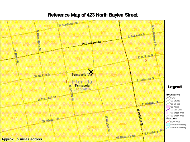
Scale: 1 inch = 440 feet (approx) or 1:5000 (approx) (Map
scale is correct when viewed at 1024 x 768 pixels at 96 DPI. The map will appear
smaller or larger when on display devices with different configurations.)
Figure 1: Reference Map of Location of Family Home in
Pensacola Florida. Census Tract 1, Block 1, Congressional District
1 (106th Congress); Source: U.S. Bureau of the Census (2003).
American FactFinder.
Figure 1: The reference map shown above depicts the location of my family home in the town of Pensacola, Florida, centered on my family home address of "423 North Baylen St." It was created using the US Census Bureau American FactFinder Web Mapping Tool located at: American Factfinder (US Census 2005) website, using the "Reference Maps" option under the "Maps" option located on the left of the screen. Having selected Maps>Reference Maps>2005 Cities and Towns (dataset option) I chose to enter the 5 digit zipcode to zoom into the city. At this point, one of the options is to "Reposition (recenter) on Address". The dataset used is the "2005 Cities and Towns". Typing in "423 North Baylen St", and "32501", the map above was returned as a result. It shows the approximate scale of the map, shows many features listed in the legend immediately to the left. Among the features detailed that show a clear delineation are "Major Roads." (Note: The 2005 Cities and Towns" dataset is an updated subset of the US Census TIGER data.)
The approximate map scale of 1":440' was derived by measuring the graphic image using JRuler, version 3.0 (Spadix 2005), and calculating the scale based on the total width as reported by American Factfinder in the graphic itself. The width of the image is very close to 6 inches. For the reported 0.5 miles for the map width extent, this equals in inches:
(0.5 miles)(5280 ft/mile)(12 inches/ft) = is equivalent to 31680 inches. (Note the dimensions cancel to inches only).
The ratio then of 6:31680 can be converted , providing a ratio of 1:5280, or 1 inch = 440 feet. Rounding down for measurement accuracy, we will call it 1:5000.
The boundaries and features shown on the map above include roads and streets, census blocks, block groups and tracts. State and County labels are included on for labeling purposes but are far outside the extent of the map to add any meaningful context. Labels are displayed for block groups, census tracts and street and road names. In addition, a label associated with a placename is provided for Pensacola, with an additional label of "UA" for "Urban Area." The house I grew up in located on the SW corner of the intersection of N Baylen St and W la Rua St. in the southern part of the county and it's location is marked with an "X". Much of my analysis will be centered on that section of the county as a result. Many of the names in this part of Pensacola are originally Spanish and date at least from the 1820's, when Florida was annexed from the Spanish Empire by General Andrew Jackson, who also served as the first US territorial Governor, ruling the new territory from Pensacola.
Figure 2 provides a reference for the location of Figure 1 within the greater Metropolitan area of Escambia County, Florida, along the Northern Gulf Coast. The area in Figure 1 is located in Escambia County, Florida, Census Tract 1, Block 1, Congressional District 1 (106th Congress).
Reference Map of Area in Figure 1
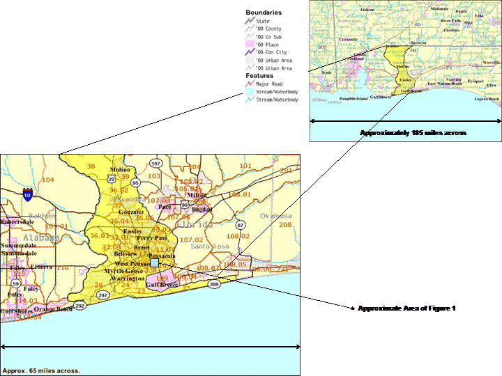
Figure 2 - Reference of Location of Figure 1 map within Escambia County and along the Northern Gulf Coast. Source: U.S. Bureau of the Census (2003). American FactFinder. Created using PowerPoint.
Table 1: Mini-Atlas of Demographic Data Regarding Escambia County Florida (derived from TIGER data files on American Factfinder of US Census Bureau)
| Map Sheet Number | Name of Map | Analysis |
| 1 | Total Persons in Escambia County Florida as of 2000. | This choropleth shows a distribution of the population of Escambia County Florida. The areas have been divided into areas that show the number of persons living in Census Blocks as of the year 2000. From the distribution it is obvious that most of the population of Escambia County resides in the southern half of the County. There are 4 data classes that reflect the raw count in each of the areas. The NW sector of the county is the most sparsely populated. |
| 2 | Persons per Square Mile as of 2000 | This choropleth map displays the population density for Escambia County Florida in persons/sqmile. It can be seen from this map that as of the year 2000, the population density is higher in the southern part of the county. Most of the population is located in the southern part of the county (see Map 1) and there are more people per square mile as well. The data classes are the same as Map 1 for consistency in the analysis. |
| 3 | Total Households as of 2000 | The number of households is greater in the southern part of the county (area in green, value = 90143). From Maps1 and 2 we saw a greater number of persons and a greater population density. Map 3 is consistent with Maps 1 and 2, but with adds context beyond the raw count of population. |
| 4 | Percentage of Persons Living in Urban Areas as Distributed in Escambia County as of 2000. | The data distribution shown in this map is consistent with Map 1 (Total Persons) Rather than raw count the percentages living in the urban areas are shown. While much could be inferred from Map 1, the percentages show a finer level of detail by showing that almost 98% of the county population lives in the southern part of the County, which is considered an urban area (UA) by the US Census Bureau |
| 5 | Median Age of Persons In Escambia County as of 2000 | The map shows the
distribution of the population by Median age. While there are
differences between the various areas shown, not enough information is
provided to determine whether the differences are statistically significant,
since no measure of variation is included. (No measure of variation is noted
in the map products from the census data.) One thing that can be noted -
from Maps 1-4, showing the vast majority of the population lived in the
southern part of the county, they seem to be younger in the southern region
as well. In otherwords, if a statistically significant difference does
exist, it is more likely it exists between the southern and northwestern
portions of the county.
Note: The median is a measure of central tendency that makes no assumptions with regards to the distribution of the underlying population. |
| 6 | Total Housing Units in Escambia as of 2000 | The map shows the distribution of the raw count of housing units in Escambia County as of the year 2000. From the map it can be determined that there are more housing units available in the southern portion of the county. |
| 7 | Percent of Housing Units Vacant as of 2000 | From Map 6 we saw that most of the housing units were in the southern region of the county. This map shows that although the number of units is higher, the vacancy rate for the southern region is much higher as well. |
| 8 | Average Family Size as of 2000 | The map above shows average family size as of 2000. While there are differences in the numbers from area to area, whether the numbers are statistically significantly different cannot be determined by the data as shown. |
| 9 | Percent of Households With One Person: 2000 | The map shows the percent of households with only one person. With respect to data from Maps 1-8, we can see that not only is the population of the southern region younger, but it tends towards a higher number of single households as well. |
| 10 | Males per 100 Females 18 Years and Over 2000 | From the map, we can see that in the southern region of the county, there are only 91 males per 100 females. This is inversely related to the northern portion of the county. The southern part of the county is more heavily populated, younger and has a higher incidence of single households. If birthrate is constant across the county, it might imply a high rate of migration of younger females from the northern rural part of the county to the more densely settled southern part of the county. Reasons might be many, but there might be more opportunity for employment and education in the southern part of the county for younger single females. |
Table 1: The 10 Thematic Maps in the "Mini-Atlas" show and describe some of the population demographics about the area I grew up in. An individual analysis follows at the bottom of each map. In general, choropleth maps use a gradient of color to represent attribute data, where the lightest area represents one end of the attribute range and the darkest the farthest attribute range of the scale. I chose to save the result as a PDF file rather than just saving the images. This preserves the full context of the source of the data, and lends itself to creating a "map book" or an atlas. All of the data is drawn from subsets of the 2000 census of Escambia County. To quote the Help Page from the Factfinder url, "Thematic Maps show interesting facts about places by using colors or patterns to shade areas on the map. You use Thematic Maps when you want to see statistical data, such as population or median income, displayed on a map." (Factfinder, US Census). This is in agreement with the text that describes Thematic Maps the same way. (DiBiase 2007). There is a short analysis for each map in the atlas included at the bottom. The text was added using Adobe Professional into the body of the pdf saved from the website.
Scale of Maps in Atlas - All of the maps in the atlas are approximately 6.19 inches across and all have the same scale. All were created using the same level of detail in the online tool and it reports all of he images as being approximately 65 miles across at the block group level. All of the thematic choropleth maps are created by combining TIGER/Line file data and 2000 census data.
(65 miles)(5280 ft/mile)(12 in/ft) = 4118400 inches. The ratio of 6.19:4118400 yields a scale of 1:665331, which for our purposes can be rounded to 1:660000. It is noted in all of the maps in the atlas. (This map scale is correct when viewed at 1024 x 768 pixels at 96 DPI. The map will appear smaller or larger when on display devices with different configurations.)
Additional data as well as another mapping tool is available from Fedstats located at http://www.fedstats.gov/qf/states/12/12033.html. It calls itself "The gateway to statistics from over 100 U.S. Federal agencies". A full explanation can be seen on http://www.fedstats.gov/aboutfedstats.html , but in general, the Federal Government has a reporting requirement for any Federal organization with expenditures of over $500,000. The current list of agencies is located at http://www.fedstats.gov/agencies and the US Census is one of those agencies. The main page is located at http://www.fedstats.gov/ . Data sets for Escambia County, can be downloaded from Browse data sets for Escambia County. One thing that is notable is the minor changes in the absolute total population of Escambia between 2000 and 2005, i.e. less than 3000 total. (Population, percent change, April 1, 2000 to July 1, 2005 = 0.8%
Personal Note: I particularly enjoyed the sections on surveying in this module. There was an interesting article on NPR the week this lesson was active and discussed a topic called Gunter's Chain and it's origin. It was a common tool used in surveying well up until the late 19th century and in fact was written in law (at least in 1785) that it had to be used for all official Government survey work. It was invented by an English mathematician named Edmund Gunter. There is a description of it in depth on http://Answers.com, but basically:
"The chain that was in common use for surveying, was 22 yards long and is divided into 100 links, each 7.92 inches in length. An acre was defined by 10 chains (or one furlong) by one chain; 100 links by 1000 links - 100,000 square links; 220 yards by 22 yards - 4840 square yards." Gunter’s link is 1 chain/100. Thus it is exactly 7.92 inches or 201.168 mm. A square link is exactly one hundred-thousandth of an acre and one ten-thousandth of one square chain or 0.0404685642 m². It is about 62¾ square inches.
Note: The links in the quotes will lead back to the exact pages for greater detail.
Sources:
Answers.com (2007) Edmund Gunter Definition and Much More from Answers_com.htm; http://Answers.com; accessed on February 15, 2007.
DiBiase, David (2007) Census Data and Thematic Maps. The Pennsylvania State University World Campus Certificate Program in GIS. Accessed February 15, 2007.
FedStats (2003). Retrieved February 24, 2007, from http://www.fedstats.gov/qf/states/12/12033.html.
Spadix Software (2004) JR Free Tools, Screen Ruler. http://www.spadixbd.com/freetools/jruler.htm Accessed February 24, 2007.
U.S. Bureau of the Census (2003). American FactFinder. Retrieved January 22, 2007, from http://factfinder.census.gov/ .
U.S. Census Bureau (2001) TIGER/Line Metadata http://www.census.gov/geo/www/tlmetadata/metadata.html Accessed February 24, 2007.
This document is published in fulfillment of an assignment by a student enrolled in an educational offering of The Pennsylvania State University. The student, named above, retains all rights to the document and responsibility for its accuracy and originality.